Conceptual Introduction
plenoptic is a python library for “model-based synthesis of perceptual
stimuli”. If you’ve never heard this phrase before, it may seem mysterious: what
is stimulus synthesis and what types of scientific investigation does it
facilitate?
Synthesis is a framework for exploring models by using them to create new
stimuli, rather than examining their responses to existing ones. plenoptic
focuses on models of visual [1] information processing, which take an image as
input, perform some computations based on parameters, and return some
vector-valued abstract representation as output. This output can be mapped to
neuronal firing rate, fMRI BOLD response, behavior on some task, image category,
etc., depending on the researchers’ intended question.

Fig. 1 Schematic describing relationship between simulate, fit, and synthesize.
That is, computational models transform a stimulus \(s\) to a response \(r\) (we often refer to \(r\) as “the model’s representation of \(s\)”), based on some model parameters \(\theta\). For example, a trained neural network that classifies images has specific weights \(\theta\), accepts an image \(s\) and returns a one-hot vector \(r\) that specifies the image class. Another example is a linear-nonlinear oriented filter model of a simple cell in primary visual cortex, where \(\theta\) defines the filter’s orientation, size, and spatial frequency, the model accepts an image \(s\) and returns a scalar \(r\) that represents the neuron’s firing rate.
The most common scientific uses for a model are to simulate responses or to fit parameters, as illustrated in Fig. 1. For simulation, we hold the parameters constant while presenting the model with inputs (e.g, photographs of dogs, or a set of sine-wave gratings) and we run the model to compute responses. For fitting, we use optimization to find the parameter values that best account for the observed responses to a set of training stimuli. In both of these cases, we are holding two of the three variables (\(r\), \(s\), \(\theta\)) constant while computing or estimating the third. We can do the same thing to generate novel stimuli, \(s\), while holding the parameters and responses constant. We refer to this process as synthesis and it facilitates the exploration of input space to improve our understanding of a model’s representations.
This is related to a long and fruitful thread of research in vision science that focuses on what humans cannot see, that is, the information they are insensitive to. Perceptual metamers — images that are physically distinct but perceptually indistinguishable — provide direct evidence of such information loss in visual representations. Color metamers were instrumental in the development of the Young-Helmholtz theory of trichromacy [Helmholtz1852]. In this context, metamers demonstrate that the human visual system projects the infinite dimensionality of the physical signal to three dimensions.
To make this more concrete, let’s walk through an example. Humans can see visible light, which is electromagnetic radiation with wavelengths between 400 and 700 nanometers (nm). We often want to be able to recreate the colors in a natural scene, such as when we take a picture. In order to do so, we can ask: what information do we need to record in order to do so? Let’s start with a solid patch of uniform color. If we wanted to recreate the complete energy spectra of the color, we would need to record a lot of numbers: even if we subsampled the wavelengths so that we only recorded the energy every 5 nm, we would need 61 numbers per color! But we know that most modern electronic screens only use three numbers, often called RGB (red, green, and blue) — why can we get away with throwing away so much information? Trichromacy and color metamers can help explain.
Researchers studying color perception arrived at a standard procedure – the bipartite color-matching experiment – for constraining a model for trichromatic metamers, illustrated in Fig. 2. An observer matches a monochromatic test color (i.e., a light with energy at only a single wavelength) with the physical mixture of three different monochromatic stimuli, called primaries. Thus, the goal is to create two perceptually-indistinguishable stimuli (metamers). Perhaps surprisingly, not only is this possible for any test color, it is also possible for just about any selection of primaries (as long as they’re within the visible light spectrum and sufficiently different from each other). For most human observers, three primaries are required: there are many colors that cannot be matched with only two primaries, and four yields non-unique responses. However, there are some people, for whom two primaries are sufficient.

Fig. 2 Color matching experiment
Requiring three primaries for most people, but two for some provided a hint regarding the underlying mechanisms: most people have cone photorecpetors from three distinct classes (generally referred to as S, M, and L, for “short”, “medium”, and “long”). But some forms of color blindness arise from genetic deviations in which only two classes are represented. Color metamers are created when cone responses have been matched. Human cones transform colors from a high-dimensional space (i.e., a vector describing the energy at each wavelength) to a three-dimensional one (i.e., a vector describing how active each cone class is). This means a large amount of wavelength information is discarded.
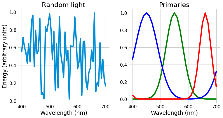
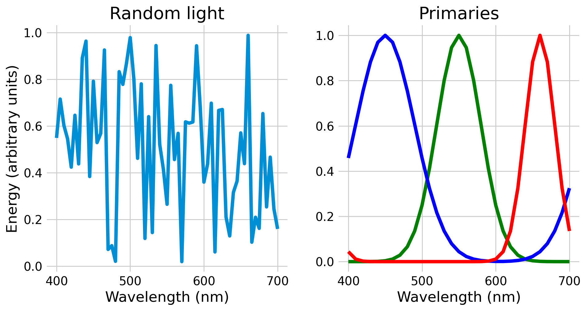
A worked example may help demonstrate this point more clearly. Let’s match the random light shown on the left below using the primaries shown on the right.
(Source code, png, hires.png, pdf)

Fig. 3 Left: Random light whose appearance we will match. Right: primaries.
The only way we can change the matching light is multiply those primaries by different numbers, moving them up and down. You might look at them and wonder how we can match the light shown on the left, with all its random wiggles. The important point is that we will not match those wiggles. We will instead match the cone activation levels, which we get by matrix multiplying our light by the cone fundamentals, shown below.
(Source code, png, hires.png, pdf)
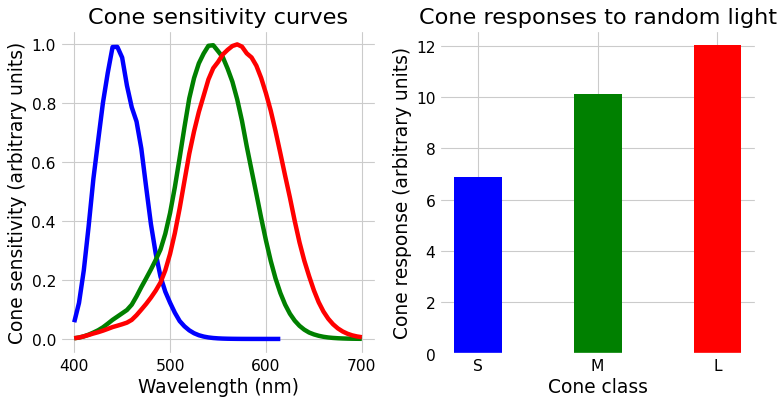
Fig. 5 Left: the cone sensitivity curves. Right: the response of each cone class to the random light shown in the previous figure.
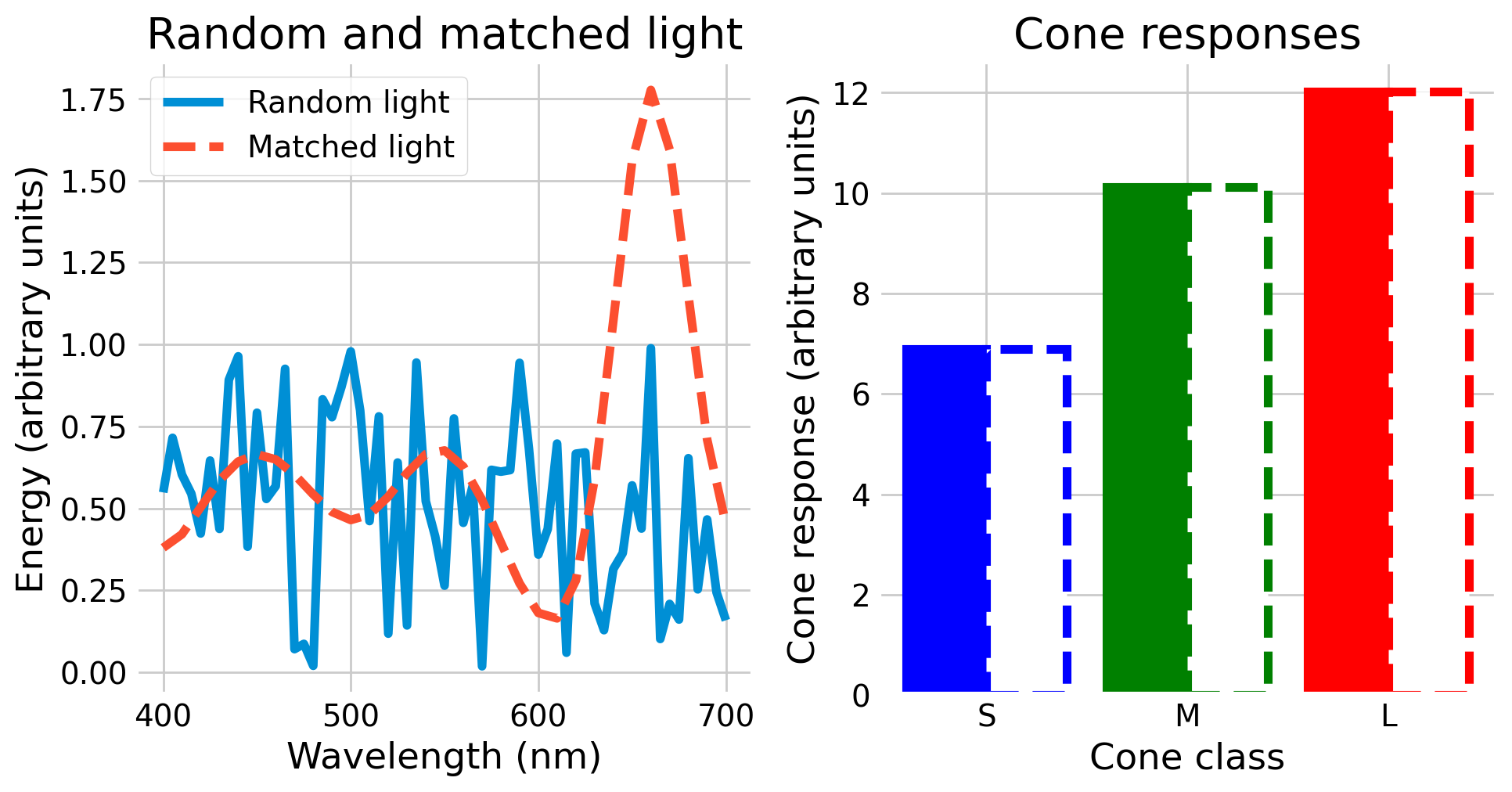
With some linear algebra, we can compute another light that has very different amounts of energy at each wavelength but identical cone responses, shown below.
(Source code, png, hires.png, pdf)

If we look at the plot on the left, we can see that the two lights are very different physically, but we can see on the right that they generate the same cone responses and thus would be perceived identically.
In this example, the model was a simple linear system of cone responses, and thus we can generate a metamer, a physically different input with identical output, via some simple linear algebra. Metamers can be useful for understanding other systems as well, because discarding information is useful: the human visual system is discarding information at every stage of processing, not just at the cones’ absorption of light, and any computational system that seeks to classify images must discard a lot of information about unnecessary differences between images in the same class. However, generating metamer for other systems gets complicated: when a system gets more complex, linear algebra no longer suffices.
Let’s consider a slightly more complex example. Human vision is very finely detailed at the center of gaze, but gradually discards this detailed spatial information as distance to the center of gaze increases. This phenomenon is known as foveation, and can be easily seen by the difficulty in reading a paragraph of text or recognizing a face out of the corner of your eye (see [Lettvin1976] for an accessible discussion with examples). The simplest possible model of foveation would be to average pixel intensities in windows whose width grows linearly with distance from the center of an image, as shown in Fig. 7:

Fig. 7 The foveated pixel intensity model averages pixel values in elliptical windows that grow in size as you move away from the center of the image. It only cares about the average in these regions, not the fine details.
This model cares about the average pixel intensity in a given area, but doesn’t care how that average is reached. If the pixels in one of the ellipses above all have a value of 0.5, if they’re half 0s and half 1s, if they’re randomly distributed around 0.5 — those are all identical, as far as the model is concerned. A more concrete example is shown in Fig. 8:

Fig. 8 Three images that the foveated pixel intensity model considers identical. They all have the same average pixel values within the foveated elliptical regions (the red ellipse shows an example averaging region at that location), but differ greatly in their fine details.
These three images are all identical for the foveated pixel intensity model described above (the red ellipse shows the size of the averaging region at that location). These three images all have identical average pixel intensities in small regions whose size grows as they move away from the center of the image. However, like the color metamers discussed earlier, they are all very physically different: the leftmost image is a natural image, the rightmost one has lots of high-frequency noise, while the center one looks somewhat blurry. You might think that, because the model only cares about average pixel intensities, you can throw away all the fine details and the model won’t notice. And you can! But you can also add whatever kind of fine details you’d like, including random noise — the model is completely insensitive to them.
With relatively simple linear models like human trichromacy and the foveated pixel intensity model, this way of thinking about models may seem unnecessary. But it is very difficult to understand how models will perform on unexpected or out-of-distribution data! The burgeoning literature on adversarial examples and robustness in machine learning provides many of examples of this, such as the addition of a small amount of noise (invisible to humans) changing the predicted category [Szegedy2013] or the addition of a small elephant to a picture completely changing detected objects’ identities and boundaries [Rosenfeld2018]. Exploring model behavior on all possible inputs is impossible — the space of all possible images is far too vast — but image synthesis provides one mechanism for exploration in a targeted manner.
Furthermore, image synthesis provides a complementary method of comparing models to the standard procedure. Generally, scientific models are evaluated on their ability to fit data or perform a task, such as how well a model performs on ImageNet or how closely a model tracks firing rate in some collected data. However, many models can perform a task equally or comparably well [2]. By using image synthesis to explore models’ representational spaces, we can gain a fuller understanding of how models succeed and how they fail to capture the phenomena under study.
Beyond Metamers
plenoptic contains more than just metamers — it provides a set of methods
for performing image synthesis. Each method allows for different exploration of
a model’s representational space:
Metamers investigate what features the model disregards entirely.
Eigendistortions investigates which features the model considers the least and which it considers the most important
Maximal differentiation (MAD) competition enables efficient comparison of two metrics, highlighting the aspects in which their sensitivities differ.
Geodesics investigates how a model represents motion and what changes to an image it considers reasonable.
The goal of this package is to facilitate model exploration and understanding.
We hope that providing these tools helps tighten the model-experiment loop: when
a model is proposed, whether by importing from a related field or
earlier experiments, plenoptic enables scientists to make targeted
exploration of the model’s representational space, generating stimuli that will
provide the most information. We hope to help theorists become more active
participants in directing future experiments by efficiently finding new
predictions to test.
Helmholtz, H. (1852). LXXXI. on the theory of compound colours. The London, Edinburgh, and Dublin Philosophical Magazine and Journal of Science, 4(28), 519–534. http://dx.doi.org/10.1080/14786445208647175
Lettvin, J. Y. (1976). On Seeing Sidelong. The Sciences, 16(4), 10–20. http://jerome.lettvin.com/jerome/OnSeeingSidelong.pdf
Szegedy, C., Zaremba, W., Sutskever, I., Bruna, J., Erhan, D., Goodfellow, I., & Fergus, R. (2013). Intriguing properties of neural networks. https://arxiv.org/abs/1312.6199
Rosenfeld, A., Zemel, R., & Tsotsos, J.~K. (2018). The elephant in the room. https://arxiv.org/abs/1808.03305